Joining data

Code for Quiz 6, more dplyr and our first interactive chart using echarts4r.

Step 1-6

1. Load the R packages we will use.

library(tidyverse)
library(echarts4r) 
library(hrbrthemes)

2. Read the data in the files drug_cos.csv, health_cos.csv in to R and assign to the variables drug_cos and health_cos`, respectively.

drug_cos <- read_csv("https://estanny.com/static/week6/drug_cos.csv")
health_cos <- read_csv("https://estanny.com/static/week6/health_cos.csv")

3. Use glimpse to get a glimpse of the data

drug_cos %>% glimpse()

Rows: 104
Columns: 9
$ ticker       <chr> "ZTS", "ZTS", "ZTS", "ZTS", "ZTS", "ZTS", "Z...
$ name         <chr> "Zoetis Inc", "Zoetis Inc", "Zoetis Inc", "Z...
$ location     <chr> "New Jersey; U.S.A", "New Jersey; U.S.A", "N...
$ ebitdamargin <dbl> 0.149, 0.217, 0.222, 0.238, 0.182, 0.335, 0....
$ grossmargin  <dbl> 0.610, 0.640, 0.634, 0.641, 0.635, 0.659, 0....
$ netmargin    <dbl> 0.058, 0.101, 0.111, 0.122, 0.071, 0.168, 0....
$ ros          <dbl> 0.101, 0.171, 0.176, 0.195, 0.140, 0.286, 0....
$ roe          <dbl> 0.069, 0.113, 0.612, 0.465, 0.285, 0.587, 0....
$ year         <dbl> 2011, 2012, 2013, 2014, 2015, 2016, 2017, 20...

health_cos %>%  glimpse()

Rows: 464
Columns: 11
$ ticker      <chr> "ZTS", "ZTS", "ZTS", "ZTS", "ZTS", "ZTS", "ZT...
$ name        <chr> "Zoetis Inc", "Zoetis Inc", "Zoetis Inc", "Zo...
$ revenue     <dbl> 4233000000, 4336000000, 4561000000, 478500000...
$ gp          <dbl> 2581000000, 2773000000, 2892000000, 306800000...
$ rnd         <dbl> 427000000, 409000000, 399000000, 396000000, 3...
$ netincome   <dbl> 245000000, 436000000, 504000000, 583000000, 3...
$ assets      <dbl> 5711000000, 6262000000, 6558000000, 658800000...
$ liabilities <dbl> 1975000000, 2221000000, 5596000000, 525100000...
$ marketcap   <dbl> NA, NA, 16345223371, 21572007994, 23860348635...
$ year        <dbl> 2011, 2012, 2013, 2014, 2015, 2016, 2017, 201...
$ industry    <chr> "Drug Manufacturers - Specialty & Generic", "...

4. Which variables are the same in both data sets

names_drug <- drug_cos %>% names()
names_health <- health_cos %>% names()
intersect(names_drug, names_health)

[1] "ticker" "name"   "year"  

5. Select subset of variables to work with

• For drug_cos select (in this order): ticker, year, grossmargin

• Extract observations for 2018

• Assign output to drug_subset

• For health_cos select (in this order): ticker , year, revenue, go, industry

• Extract observations for 2018

• Assign output to health_subset

drug_subset <- drug_cos %>% 
  select(ticker, year, grossmargin) %>% 
  filter(year == 2018)

health_subset <- health_cos %>% 
  select(ticker, year, revenue, gp, industry) %>% 
  filter(year == 2018)

6. Keep all the rows and columns drug_subset join with column in health_subset

drug_subset %>% left_join(health_subset)

# A tibble: 13 x 6
   ticker  year grossmargin   revenue        gp industry              
   <chr>  <dbl>       <dbl>     <dbl>     <dbl> <chr>                 
 1 ZTS     2018       0.672   5.82e 9   3.91e 9 Drug Manufacturers - ~
 2 PRGO    2018       0.387   4.73e 9   1.83e 9 Drug Manufacturers - ~
 3 PFE     2018       0.79    5.36e10   4.24e10 Drug Manufacturers - ~
 4 MYL     2018       0.35    1.14e10   4.00e 9 Drug Manufacturers - ~
 5 MRK     2018       0.681   4.23e10   2.88e10 Drug Manufacturers - ~
 6 LLY     2018       0.738   2.46e10   1.81e10 Drug Manufacturers - ~
 7 JNJ     2018       0.668   8.16e10   5.45e10 Drug Manufacturers - ~
 8 GILD    2018       0.781   2.21e10   1.73e10 Drug Manufacturers - ~
 9 BMY     2018       0.71    2.26e10   1.60e10 Drug Manufacturers - ~
10 BIIB    2018       0.865   1.35e10   1.16e10 Drug Manufacturers - ~
11 AMGN    2018       0.827   2.37e10   1.96e10 Drug Manufacturers - ~
12 AGN     2018       0.861   1.58e10   1.36e10 Drug Manufacturers - ~
13 ABBV    2018       0.764   3.28e10   2.50e10 Drug Manufacturers - ~

Question: join ticker

• Start with drug_cos

• Extract observations for the ticker BIIB from drug_cos

• Assign output to the variable drug_cos_subset

drug_cos_subset <- drug_cos %>% 
  filter(ticker == "BIIB")

---

• Display drug_cos_subset

 drug_cos_subset

# A tibble: 8 x 9
  ticker name  location ebitdamargin grossmargin netmargin   ros   roe
  <chr>  <chr> <chr>           <dbl>       <dbl>     <dbl> <dbl> <dbl>
1 BIIB   Biog~ Massach~        0.404       0.908     0.245 0.333 0.204
2 BIIB   Biog~ Massach~        0.402       0.901     0.25  0.335 0.211
3 BIIB   Biog~ Massach~        0.432       0.876     0.269 0.355 0.233
4 BIIB   Biog~ Massach~        0.475       0.879     0.302 0.404 0.294
5 BIIB   Biog~ Massach~        0.493       0.885     0.33  0.437 0.321
6 BIIB   Biog~ Massach~        0.491       0.871     0.323 0.431 0.322
7 BIIB   Biog~ Massach~        0.495       0.867     0.207 0.407 0.209
8 BIIB   Biog~ Massach~        0.511       0.865     0.329 0.435 0.334
# ... with 1 more variable: year <dbl>

• Use left_join to combine the rows and columns of drug_cos_subset with the columns of health_cos

• Assgin the output to combo_df

combo_df <- drug_cos_subset %>% 
  left_join(health_cos)

---

• Display combo_df

combo_df

# A tibble: 8 x 17
  ticker name  location ebitdamargin grossmargin netmargin   ros   roe
  <chr>  <chr> <chr>           <dbl>       <dbl>     <dbl> <dbl> <dbl>
1 BIIB   Biog~ Massach~        0.404       0.908     0.245 0.333 0.204
2 BIIB   Biog~ Massach~        0.402       0.901     0.25  0.335 0.211
3 BIIB   Biog~ Massach~        0.432       0.876     0.269 0.355 0.233
4 BIIB   Biog~ Massach~        0.475       0.879     0.302 0.404 0.294
5 BIIB   Biog~ Massach~        0.493       0.885     0.33  0.437 0.321
6 BIIB   Biog~ Massach~        0.491       0.871     0.323 0.431 0.322
7 BIIB   Biog~ Massach~        0.495       0.867     0.207 0.407 0.209
8 BIIB   Biog~ Massach~        0.511       0.865     0.329 0.435 0.334
# ... with 9 more variables: year <dbl>, revenue <dbl>, gp <dbl>,
#   rnd <dbl>, netincome <dbl>, assets <dbl>, liabilities <dbl>,
#   marketcap <dbl>, industry <chr>

• Note: the variable ticker, name, location and industry are the same for all the observations

---

• Assign the company name to co_name

co_name <- combo_df %>% 
  distinct(name) %>% 
  pull()

---

• Assign the company location to co_location

co_location <- combo_df %>% 
  distinct(location) %>% 
  pull()

---

• Assign the industry to co_industry group

co_industry <- combo_df %>% 
  distinct(industry) %>% 
  pull

Put the r inline commands used in the blanks below. When yo knit the document the results of the commands will be displayed in your text. The company Biogen Inc is located in Massachusetts; U.S.A and is a member of the Drug Manufacturers - General industry group.

---

• Start with combo_df

• Select variables (in this order): year, grossmargin, netmargin, revenue, gp, netincome

• Assign the output to combo_df_subset

combo_df_subset <-  combo_df %>% 
  select(year, grossmargin, netmargin, revenue, gp, netincome)

---

• Display combo_df_subset

combo_df_subset

# A tibble: 8 x 6
   year grossmargin netmargin     revenue          gp  netincome
  <dbl>       <dbl>     <dbl>       <dbl>       <dbl>      <dbl>
1  2011       0.908     0.245  5048634000  4581854000 1234428000
2  2012       0.901     0.25   5516461000  4970967000 1380033000
3  2013       0.876     0.269  6932200000  6074500000 1862300000
4  2014       0.879     0.302  9703300000  8532300000 2934800000
5  2015       0.885     0.33  10763800000  9523400000 3547000000
6  2016       0.871     0.323 11448800000  9970100000 3702800000
7  2017       0.867     0.207 12273900000 10643900000 2539100000
8  2018       0.865     0.329 13452900000 11636600000 4430700000

---

• Create the variable grossmargin_check to compare with the variable grossmargin. They should be equal
  • grossmargin_check = gp / revenue
• Create the variable cloase_enough to check that the absolute value of the difference between grossmargin_check and grossmargin is less than 0.001

combo_df_subset %>% 
  mutate(grossmargin_check = gp/revenue,
         close_enough = abs(grossmargin-grossmargin)< 0.001)

# A tibble: 8 x 8
   year grossmargin netmargin revenue      gp netincome
  <dbl>       <dbl>     <dbl>   <dbl>   <dbl>     <dbl>
1  2011       0.908     0.245 5.05e 9 4.58e 9    1.23e9
2  2012       0.901     0.25  5.52e 9 4.97e 9    1.38e9
3  2013       0.876     0.269 6.93e 9 6.07e 9    1.86e9
4  2014       0.879     0.302 9.70e 9 8.53e 9    2.93e9
5  2015       0.885     0.33  1.08e10 9.52e 9    3.55e9
6  2016       0.871     0.323 1.14e10 9.97e 9    3.70e9
7  2017       0.867     0.207 1.23e10 1.06e10    2.54e9
8  2018       0.865     0.329 1.35e10 1.16e10    4.43e9
# ... with 2 more variables: grossmargin_check <dbl>,
#   close_enough <lgl>

---

• Create the variable netmargin_check to compare with the variable netmargin. They should be equal.

• Create the variable close_enough to check that the absolute value of the difference between netmargin_check and netmargin is less than 0.001

combo_df_subset %>% 
  mutate(netmargin_check=netincome/revenue,
         close_enough=abs(netmargin_check-netmargin)<0.001)

# A tibble: 8 x 8
   year grossmargin netmargin revenue      gp netincome
  <dbl>       <dbl>     <dbl>   <dbl>   <dbl>     <dbl>
1  2011       0.908     0.245 5.05e 9 4.58e 9    1.23e9
2  2012       0.901     0.25  5.52e 9 4.97e 9    1.38e9
3  2013       0.876     0.269 6.93e 9 6.07e 9    1.86e9
4  2014       0.879     0.302 9.70e 9 8.53e 9    2.93e9
5  2015       0.885     0.33  1.08e10 9.52e 9    3.55e9
6  2016       0.871     0.323 1.14e10 9.97e 9    3.70e9
7  2017       0.867     0.207 1.23e10 1.06e10    2.54e9
8  2018       0.865     0.329 1.35e10 1.16e10    4.43e9
# ... with 2 more variables: netmargin_check <dbl>,
#   close_enough <lgl>

Question: summarize_industry

• Fill in the blanks

• Put the command you use in the Rchunks in the Rmd fo rthis quiz

• Use the health_cos data

• For each industrty calculate

  • mean_grossmargin_percent = mean(gp/revenue) * 100
  • median_grossmargin percent= median(gp/revenue) * 100
  • min_gorssmargin_percent = min(gp/revenue) * 100
  • max_grossmargin_percent = max(gp/revenue) * 100

health_cos %>% 
  group_by(industry) %>%
  summarize(mean_grossmargin_percent=mean(gp/revenue)*100,
            median_grossmargin_percent=median(gp/revenue)*100,
            min_grossmargin_percent=min(gp/revenue)*100,
            max_grossmargin_percent=max(gp/revenue)*100)

# A tibble: 9 x 5
  industry mean_grossmargi~ median_grossmar~ min_grossmargin~
* <chr>               <dbl>            <dbl>            <dbl>
1 Biotech~             92.5            92.7             81.7 
2 Diagnos~             50.5            52.7             28.0 
3 Drug Ma~             75.4            76.4             36.8 
4 Drug Ma~             47.9            42.6             34.3 
5 Healthc~             20.5            19.6             10.0 
6 Medical~             55.9            37.4             28.1 
7 Medical~             70.8            72.0             53.2 
8 Medical~             10.4             5.38             2.49
9 Medical~             53.9            52.8             40.5 
# ... with 1 more variable: max_grossmargin_percent <dbl>

• mean_grossmargin_percent for the industry Medical Devices is 70.78%

• median_grossmargin_percent for the industry Medical Devices is 71.98%

• min_grossmargin_percent for the industry Medical Devices is 53.21%

• max_grossmargin_percent for the industry Medical Devices is 84.70%

Question: inline_ticker

*Fill in the blanks

• Use the health_cos data

• Extract observations for the ticker BMY from health_cos and assign to the variable health_cos_subset

health_cos_subset <- health_cos %>% 
  filter(ticker == "BMY")

---

• Display health_cos_subset

health_cos_subset

# A tibble: 8 x 11
  ticker name  revenue      gp    rnd netincome  assets liabilities
  <chr>  <chr>   <dbl>   <dbl>  <dbl>     <dbl>   <dbl>       <dbl>
1 BMY    Bris~ 2.12e10 1.56e10 3.84e9    3.71e9 3.30e10 17103000000
2 BMY    Bris~ 1.76e10 1.30e10 3.90e9    1.96e9 3.59e10 22259000000
3 BMY    Bris~ 1.64e10 1.18e10 3.73e9    2.56e9 3.86e10 23356000000
4 BMY    Bris~ 1.59e10 1.19e10 4.53e9    2.00e9 3.37e10 18766000000
5 BMY    Bris~ 1.66e10 1.27e10 5.92e9    1.56e9 3.17e10 17324000000
6 BMY    Bris~ 1.94e10 1.45e10 5.01e9    4.46e9 3.37e10 17360000000
7 BMY    Bris~ 2.08e10 1.47e10 6.48e9    1.01e9 3.36e10 21704000000
8 BMY    Bris~ 2.26e10 1.60e10 6.34e9    4.92e9 3.50e10 20859000000
# ... with 3 more variables: marketcap <dbl>, year <dbl>,
#   industry <chr>

• In the console, type ?distinct. Go to the help pane to see what distinct does

• In the console, type ?pull. Go to the help pane to see what pull does

Run the code below

health_cos_subset %>% 
  distinct(name) %>% 
  pull(name)

[1] "Bristol Myers Squibb Co"

• Assign the output to co_name

co_name <-  health_cos_subset %>% 
  distinct(name) %>%  
  pull(name)

You can take outout from your code and include it in your text.

• The name of the company with ticker BMY is Bristol Myers Squibb Co

In following chunk * Assign the comapny’s industry group to the variable co_industry

co_industry <- health_cos_subset %>% 
  distinct(industry) %>% 
  pull()

This is outside the Rchunk. Put the r inline commands used in the blanks below. When you knit the document the results of the commands will be displayed in your text.

The company Bristol Myers Squibb Co is a member of the Drug Manufacturers - General group.

Steps 7-11

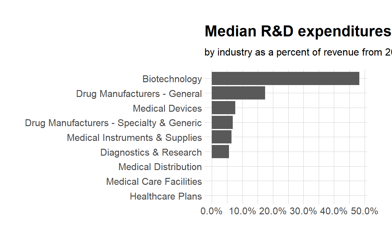
7. Prepare the data for the plots

• start with health_cos THEN
• group by industry THEN
• calculate the median research and development expenditure by industry
• assign the output to df

df <- health_cos %>% 
  group_by(industry) %>% 
  summarise(med_rnd_rev = median(rnd/revenue))

8. Use glimpse to glimpse the data for the plots

df %>% glimpse()

Rows: 9
Columns: 2
$ industry    <chr> "Biotechnology", "Diagnostics & Research", "D...
$ med_rnd_rev <dbl> 0.48317287, 0.05620271, 0.17451442, 0.0685187...

9. Create a static bar chart

• use ggplot to initiate the chart
• data is df
• the variable industry is mapped to the x-axis
  • reorder it based the value of med_rnd_rev
• the variable med_rnd_rev is mapped to the y-axis
• add a bar chart using geom_col
• use scale_y_conditions to lable the y-axis with percent
• use coord_flip() to flip the coordinates
• use labs to add title, subtitle and rename x and y-axes
• use theme_ipsum() from the hrbethemes package to improve the theme

ggplot(data = df, 
       mapping = aes(
         x = reorder(industry, med_rnd_rev ),
         y = med_rnd_rev
         )) +
  geom_col() + 
  scale_y_continuous(labels = scales::percent) +
  coord_flip() +
  labs(
    title = "Median R&D expenditures",
    subtitle = "by industry as a percent of revenue from 2011 to 2018",
    x = NULL, y = NULL) +
  theme_ipsum()

10. Save the previous plot to preview.png and add to the yaml chunk at the top

ggsave(filename = "preview.png", 
       path = here::here("_posts", "2021-03-15-joining-data"))

11. Create an interactive bar chart using the package echarts4r

• start with the data df
• use arrange to reorder med_rnd_rev
• use e_charts to initialize a chart
  • the variable industry is mapped to the x-axis
• add a bar chart using e_bar with the values of med_rnd_rev
• use e_flip_coords() to flip the coordinates
• use e_title to add the title and the subtitle
• use e_legend to remove the legends
• use e_x_axis to change format of labels on x-axis to percent
• use e_y_axis to remove labels on y-axis-
• use e_theme to change the theme. Find more themes here

df  %>% 
  arrange(med_rnd_rev)  %>%
  e_charts(
    x = industry
    )  %>% 
  e_bar(
    serie = med_rnd_rev, 
    name = "median"
    )  %>%
  e_flip_coords()  %>% 
  e_tooltip()  %>% 
  e_title(
    text = "Median industry R&D expenditures", 
    subtext = "by industry as a percent of revenue from 2011 to 2018",
    left = "center") %>% 
  e_legend(FALSE) %>% 
  e_x_axis(
    formatter = e_axis_formatter("percent", digits = 0)
    )  %>%
  e_y_axis(
    show = FALSE
  )  %>% 
  e_theme("infographic")